Learning algorithms are the methods by which computers can process and learn from data. They’re the basis of the models that are used in ML.
These algorithms can be categorised based on their functionality and the type of task they are designed for.
70.2 Basic Algorithms
Linear Regression
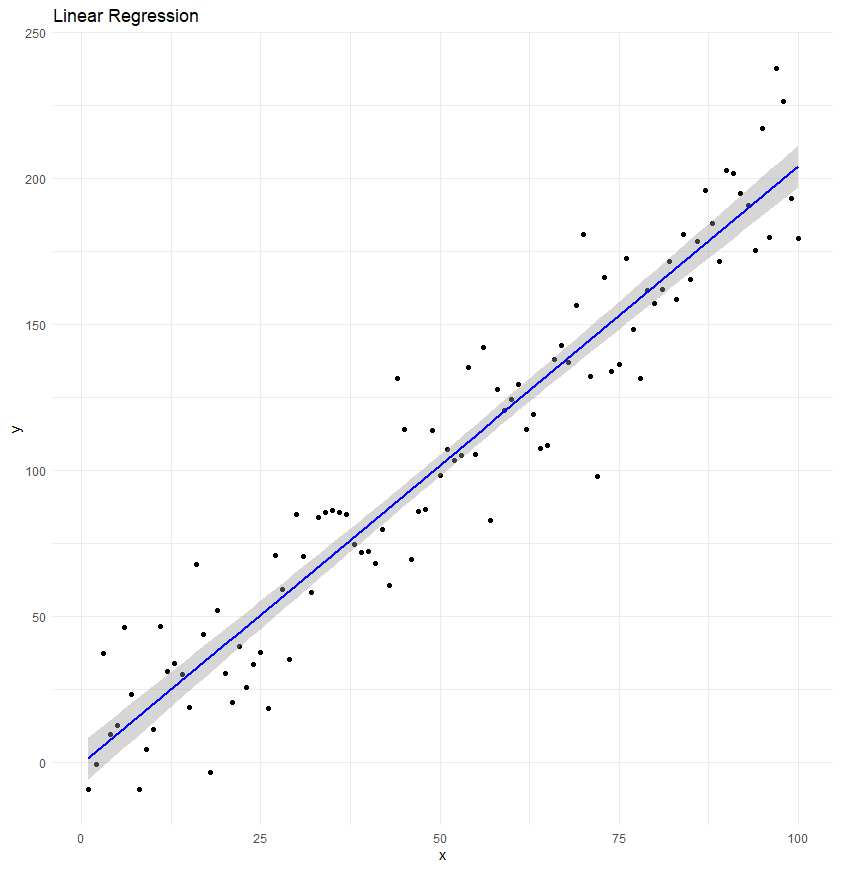
Linear regression predicts a continuousoutcome based on one or more input features. We covered these earlier in the module.
model <-lm(mpg ~ wt + hp, data = mtcars)summary(model)
Call:
lm(formula = mpg ~ wt + hp, data = mtcars)

Residuals:
   Min     1Q Median     3Q    Max
-3.941 -1.600 -0.182  1.050  5.854

Coefficients:
            Estimate Std. Error t value Pr(>|t|)
(Intercept) 37.22727    1.59879  23.285  < 2e-16 ***
wt          -3.87783    0.63273  -6.129 1.12e-06 ***
hp          -0.03177    0.00903  -3.519  0.00145 **
---
Signif. codes:  0 '***' 0.001 '**' 0.01 '*' 0.05 '.' 0.1 ' ' 1

Residual standard error: 2.593 on 29 degrees of freedom
Multiple R-squared:  0.8268,    Adjusted R-squared:  0.8148
F-statistic: 69.21 on 2 and 29 DF,  p-value: 9.109e-12
Linear regression is the simplest form of regression analysis, where the relationship between the independent variables and the dependent variable is assumed to be linear. The model predicts the dependent variable’s value as a straight-line function of the independent variable(s).
Mathematically, this is expressed as:
\[
Y=β0+β1X1+β2X2+...+βnXn+ϵ
\]
where \(Y\) is the dependent variable, \(Xi\) are the independent variables, \(βi\) are the coefficients representing the relationship’s direction and strength, and \(ϵ\) is the error term.
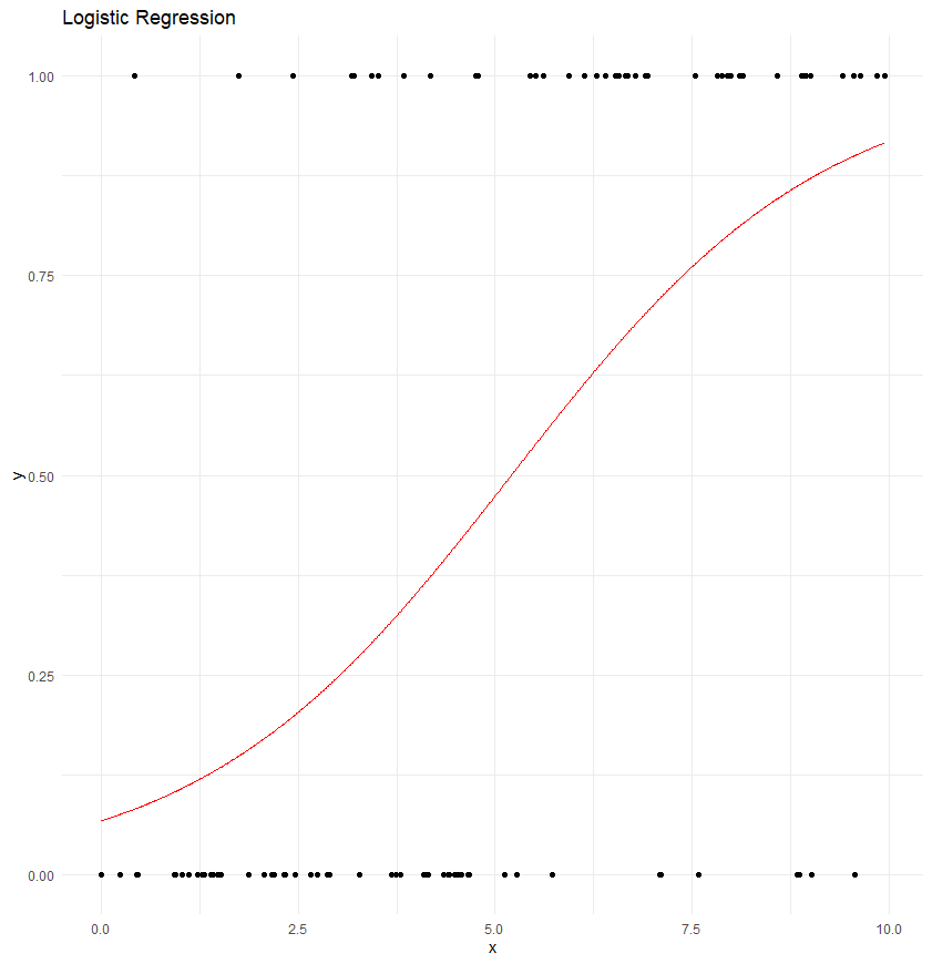
Logistic regression is used when the dependent variable is categorical, typically binary, such as 0 or 1, yes or no, true or false.
Unlike linear regression that predicts a continuous outcome, logistic regression estimates the probability of the categorical outcome based on one or more predictor variables.
The logistic function (or sigmoid function) is used to model the probability that the dependent variable belongs to a particular category. This is particularly useful in classification tasks, such as spam detection, disease diagnosis, and customer churn prediction.
Evaluating Regression Models: RMSE, MAE, R²
The performance of regression models is evaluated using various metrics to measure the difference between the observed values and the values predicted by the model.
Root Mean Squared Error (RMSE) and Mean Absolute Error (MAE) are two commonly used metrics for this purpose.
RMSE calculates the square root of the average squared differences between predicted and actual values, giving a sense of how far the predictions are from the real data points.
MAE measures the average magnitude of errors in a set of predictions, without considering their direction.
Lower values of RMSE and MAE indicate better model performance.
Another important metric is the Coefficient of Determination, denoted as R², which quantifies the proportion of the variance in the dependent variable that is predictable from the independent variables. R² values range from 0 to 1, with higher values indicating a better fit between the model and the data.
K-Nearest Neighbors
A simple algorithm that stores all available cases and classifies new cases based on a similarity measure (e.g., distance functions):
library(class)data(iris)train <-sample(1:150, 100)knn.model <-knn(train = iris[train, 1:4], test = iris[-train, 1:4], cl = iris[train, 5], k =3)table(iris[-train, 5], knn.model)
Three more complex algorithms are decision trees, neural networks, and support vector machines, each of which has a different approach and areas of application.
Decision Trees
Decision Trees are a type of learning algorithm that models decisions and their possible consequences, including chance event outcomes, resource costs, and utility.
They are a non-parametric supervised learning method used for classification and regression tasks.
More on non-parametric supervised learning methods
A non-parametric supervised learning method is a type of machine learning approach that does not make explicit assumptions about the form or parameters of the underlying function to be learned.
Unlike parametric methods, which have a fixed number of parameters and a predetermined form (like a linear equation), non-parametric methods are more flexible as they can adapt to a larger variety of data shapes and structures.
This flexibility allows them to capture more complex patterns in the data, but can also make them more prone to overfitting, especially with small data sets.
Common examples of non-parametric supervised learning methods include decision trees, k-nearest neighbors, and kernel methods. These methods are “supervised” because they learn from a dataset that contains both input features and corresponding output labels to make predictions.
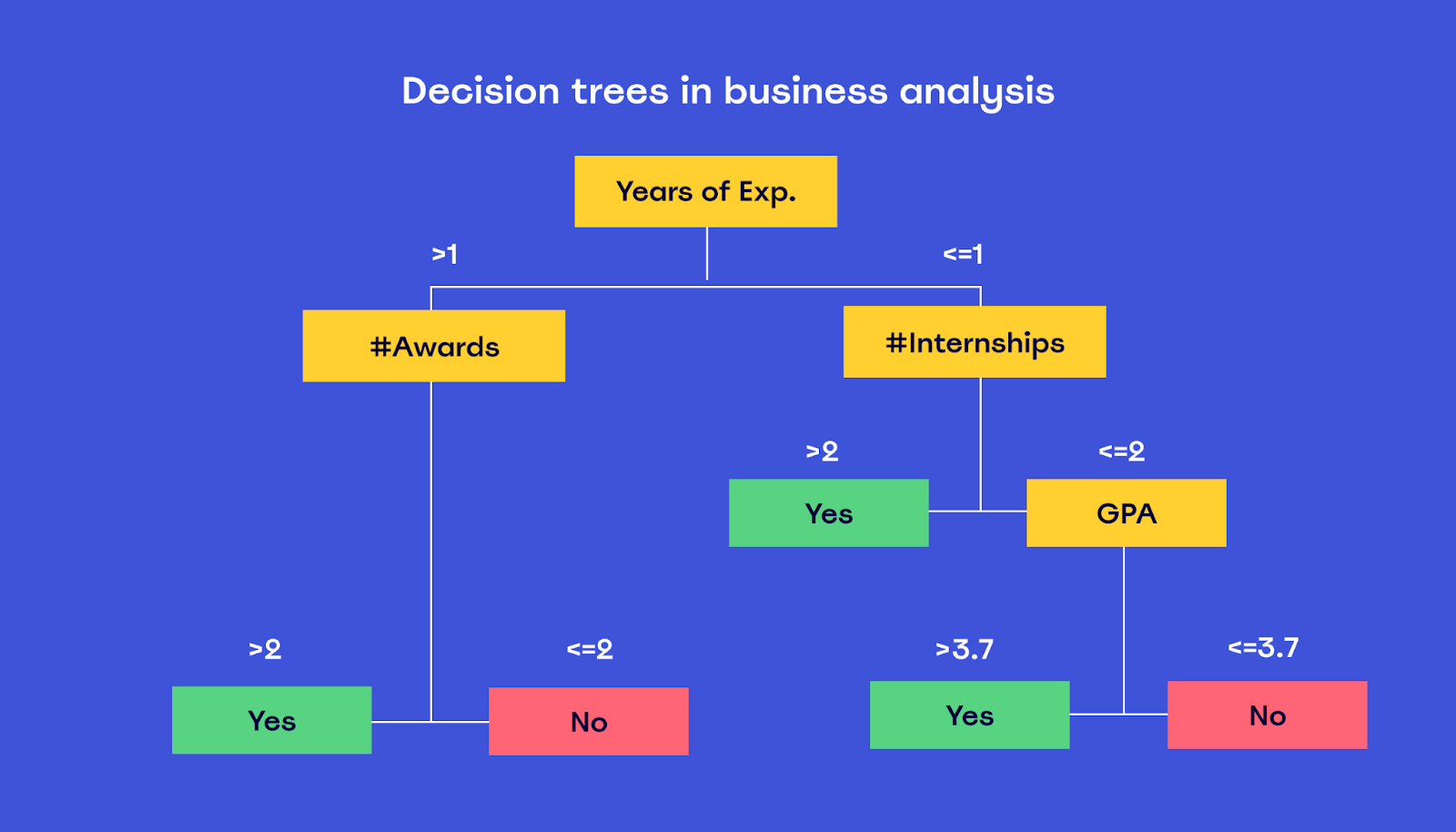
The decision tree algorithm splits the data into subsets based on the value of input variables, and this process is repeated recursively. This results in a tree-like model of decisions, where each node in the tree represents a choice between a number of alternatives, and each leaf represents a classification or decision.
library(rpart)model <-rpart(Species ~ ., data = iris, method ="class")printcp(model) # Display the results
Decision trees are particularly valued for their simplicity, interpretability, and ease of visualisation, making them accessible to non-technical users.
Neural Networks
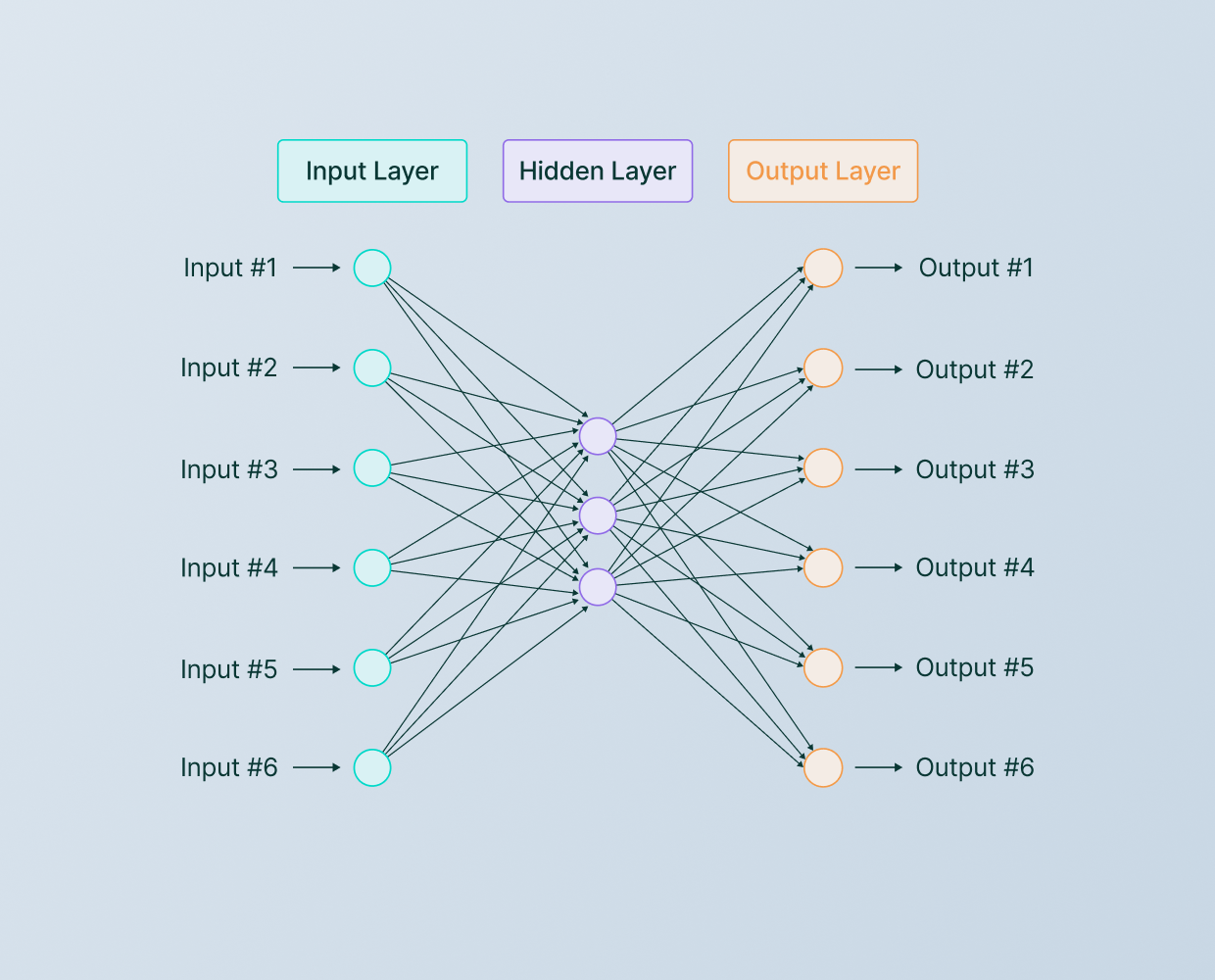
Neural Networks, inspired by the structure and function of the human brain, are a more complex learning algorithm compared to decision trees.
They consist of layers of interconnected nodes, each resembling a neuron. The nodes in each layer peSrform various transformations on their inputs before passing the signal to the next layer.
Neural networks are good at processing patterns in complex data, making them suitable for tasks like image and speech recognition, natural language processing, and even playing games at a high level. The flexibility and adaptability of neural networks come from their ability to learn to approximate any function, given enough data and computational power.
Support Vector Machines
Support Vector Machines (SVM) are another powerful and versatile supervised learning algorithm, used for both classification and regression tasks.
SVM works by finding the ‘hyperplane’ that best divides a dataset into classes.
The strength of SVM lies in its use of kernel functions, which enable it to handle non-linear data. It’s especially effective in high-dimensional spaces and in situations where the number of dimensions exceeds the number of samples.
SVMs are known for their robustness, particularly in avoiding over-fitting, and are widely used in applications ranging from handwriting recognition to cancer classification.
70.4 Evaluating Machine Learning Models
Metrics for Model Performance
Like all forms of model-building, it’s crucial to evaluate the performance of your ML models using metrics like accuracy, precision, recall, and F1 score.
For example, in the case of a binary classification problem, you can analyse the confusion matrix. Previously, we noted that this tells us how accurate our model is in its predictions (see here.
The confusion matrix and ROC curve are more advanced methods to assess the performance of your classification models. These are worth exploring further if ML is of interest to you.